Example Experiment: N170 (Face/Body)

This tutorial uses a complete example dataset to walk through the EegFun.jl analysis pipeline, focusing on the N170 component — a face-sensitive ERP that peaks around 170 ms at posterior electrodes.

The Experiment

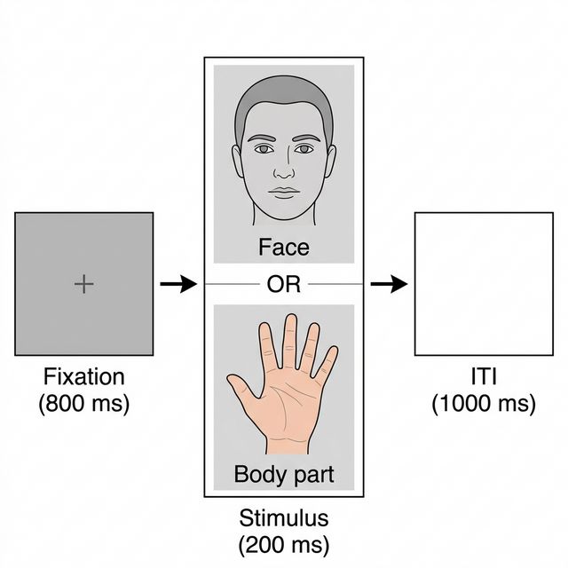
Participants passively viewed images of faces and body parts while counting images depicting an injury (task-relevant targets to maintain attention). On each trial, a fixation cross appeared for 800 ms, followed by the image for 200 ms, then a blank inter-trial interval of 1000 ms.

Experimental Design

The design is a single-factor within-subjects comparison:

Factor	Levels
Stimulus Type	Body, Face

Trigger	Category
1	Body
2	Body
3	Body
5	Face
6	Face

Data

Property	Value
Participants	10
EEG System	BioSemi ActiveTwo
Channels	66 Cap EEG + 4 EOG + 2 Mastoids (72 in total)
File Format	BDF (BioSemi Data Format)
Sample Rate	512 Hz

The N170 Component

The N170 is a negative-going ERP component peaking around 170 ms post-stimulus at posterior lateral electrodes (P7, P8, PO7, PO8). It is reliably larger for faces compared to other visual categories, making it one of the most studied markers of face-specific processing (Bentin et al., 1996).

---

Part 1: Single Participant Exploration

We start by working with a single file to explore the data, understand the preprocessing steps, and build intuition before scaling to the full dataset.

1.1 Load Raw Data

using EegFun

# Read the raw BDF file and channel layout
dat = EegFun.read_raw_data("example1.bdf")
layout = EegFun.read_layout("biosemi72.csv")

# Create the EegFun data structure
dat = EegFun.create_eegfun_data(dat, layout)

1.2 Channel Layout and Neighbours

Plot the channel layout to check that electrode positions look correct:

EegFun.plot_layout_2d(dat)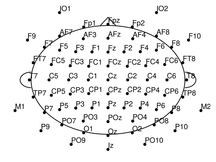

Define channel neighbours (used later for electrode repair and cluster-based statistics):

EegFun.get_neighbours_xy!(dat, 0.4)

Plot again with neighbour connections (interactive with mouse hover):

EegFun.plot_layout_2d(dat, neighbours = true)

You can also inspect the layout interactively and export the neighbour definitions:

EegFun.viewer(dat.layout)
dat.layout.neighbours
EegFun.print_layout_neighbours(layout, "./neighbours.toml")

1.3 Inspect Triggers

Check which trigger codes are present and how many of each:

EegFun.trigger_count(dat)

File: example7
Type: EegFun.ContinuousData
Labels: Fp1, AF7, AF3, F1, F3, ..., F10, IO1, IO2, M1, M2
Duration: 464.998046875 S
Sample Rate: 512

Trigger Count Summary
┌─────────┬───────┐
│ trigger │ count │
│   Int64 │ Int64 │
├─────────┼───────┤
│       1 │    36 │
│       2 │    26 │
│       3 │    26 │
│       5 │    55 │
│       6 │    55 │
│     253 │     1 │
└─────────┴───────┘

Triggers 1–3 are body stimuli and triggers 5–6 are face stimuli. Trigger 253 is a recording artefact (BioSemi status byte) and can be ignored.

Get a visual overview of the trigger distribution:

EegFun.plot_trigger_overview(dat)

Inspect trigger timing — when each trigger occurred and the interval between triggers:

EegFun.plot_trigger_timing(dat)

You should see triggers 1–3 corresponding to body images and triggers 5–6 for face images, with a regular ~2000 ms inter-trial interval (800 ms fixation + 200 ms image + 1000 ms ITI).

1.4 Browse the Raw Data

You can inspect the raw data structure directly:

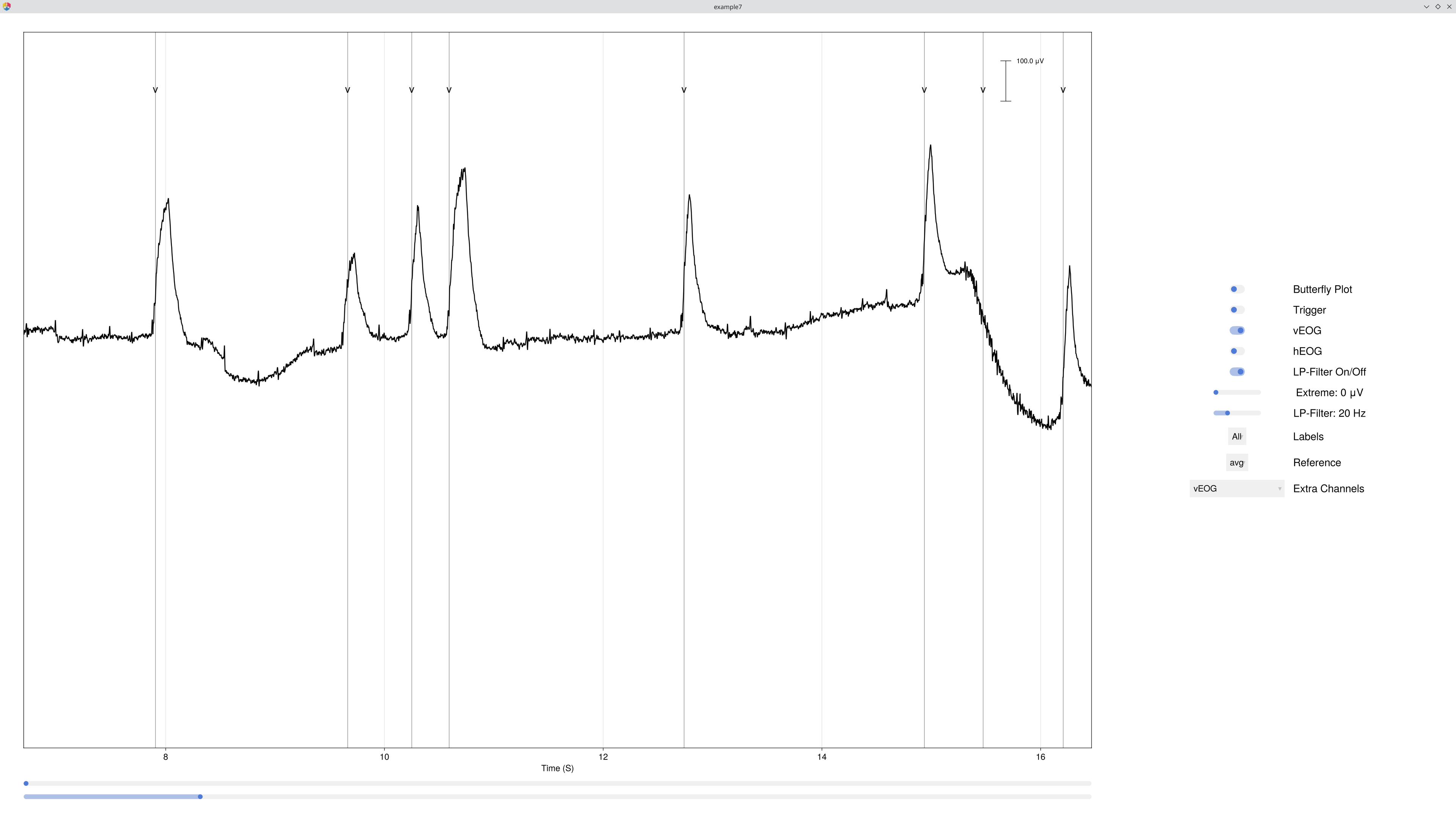
EegFun.viewer(dat)

The databrowser lets you scroll through the continuous recording and visually inspect data quality:

EegFun.plot_databrowser(dat)

Before going further, remove the DC offset with a high-pass filter and rereference to the average — this makes the traces much easier to read:

# Remove DC offset
EegFun.highpass_filter!(dat, 0.1)

# Rereference to the average of all channels
EegFun.rereference!(dat, :avg)

# Plot again to see the effect
EegFun.plot_databrowser(dat)

Look for obvious artifacts: flat channels, excessive drift, large muscle movements. This gives you a feel for data quality before automated processing.

1.5 Derive EOG Channels

The raw recording includes four EOG electrodes (IO1, IO2, F9, F10) placed around the eyes. By computing the difference between electrode pairs we get clean vertical and horizontal EOG signals that make blinks and saccades easy to spot:

# Vertical EOG: average of upper channels minus average of lower channels
EegFun.channel_difference!(
    dat,
    channel_selection1 = EegFun.channels([:Fp1, :Fp2]),
    channel_selection2 = EegFun.channels([:IO1, :IO2]),
    channel_out = :vEOG,
)
# Horizontal EOG: left minus right
EegFun.channel_difference!(
    dat,
    channel_selection1 = EegFun.channels([:F9]),
    channel_selection2 = EegFun.channels([:F10]),
    channel_out = :hEOG,
)

Next, automatically detect EOG onsets and mark the surrounding interval as contaminated. This creates Boolean columns (:is_vEOG, :is_hEOG) that the databrowser renders as shaded overlays:

EegFun.detect_eog_onsets!(dat, 50, :vEOG, :is_vEOG)
EegFun.detect_eog_onsets!(dat, 50, :hEOG, :is_hEOG)

The new :vEOG and :hEOG channels appear under the Extra Channels tab in the databrowser, so you can scroll through the recording and verify that blinks and saccades are captured correctly.

1.6 Visualise Epoch Regions

Before extracting epochs, it is useful to see where they would land on the continuous recording. mark_epoch_intervals! creates a Boolean channel that marks every sample falling within a time window around each trigger:

# Mark the epoch window (−200 ms to 1200 ms) around every stimulus trigger
EegFun.mark_epoch_intervals!(dat, [1, 2, 3, 5, 6], [-0.2, 1.2])

# Browse again — the epoch regions now appear as shaded overlays, and we can also see the EOG detection
EegFun.plot_databrowser(dat)

The highlighted regions let you quickly check whether epoch boundaries overlap, whether any epochs contain obvious artifacts, and whether the trigger timing looks correct.

1.7 Channel Quality and Extreme Values

Use channel_summary to get a quick overview of each channel's range, variance, and standard deviation — this helps spot noisy or flat channels:

# Summary across the entire recording
cs = EegFun.channel_summary(dat)
EegFun.viewer(cs)

# Summary restricted to only the epoch regions we just marked
cs_epoch = EegFun.channel_summary(dat,
    sample_selection = EegFun.samples(:epoch_interval)
)
EegFun.viewer(cs)

# Visualise with a bar chart
EegFun.plot_channel_summary(cs, :range)
EegFun.plot_channel_summary(cs, [:range, :min, :max, :var])
EegFun.plot_channel_summary(cs_epoch, :range)

Next, flag every sample where any channel exceeds ±500 μV. This creates a Boolean column (:is_extreme_value_500) that the databrowser renders as shaded overlays:

# Mark extreme samples
EegFun.is_extreme_value!(dat, 500)

# Browse — extreme-value regions now appear as red highlights
EegFun.plot_databrowser(dat)

1.8 ICA

ICA works best on data that has been high-pass filtered (e.g., ≥ 1 Hz). We copy the data, apply a stricter filter, and exclude extreme samples so the decomposition focuses on genuine brain and artifact sources:

# Copy data and apply stricter filter for ICA
dat_ica = copy(dat)
EegFun.highpass_filter!(dat_ica, 1.0)

# Run ICA, excluding bad channels
# ica_result = EegFun.run_ica(dat_ica)
# ica_result = EegFun.run_ica(dat_ica, channel_selection = EegFun.channels_not(bad_channels), sample_selection = EegFun.samples_not(:is_extreme_value_500))
ica_result = EegFun.run_ica(dat_ica, sample_selection = EegFun.samples_not(:is_extreme_value_500))

Inspect the component topographies and time-course activations:

# Component topographies
EegFun.plot_topography(ica_result, component_selection = EegFun.components(1:10));
EegFun.plot_ica_component_activation(dat, ica_result)
EegFun.plot_databrowser(dat, ica_result)

For long recordings, subsample (percentage_of_data) can be used to speed up ICA:

ica_result = EegFun.run_ica(dat_ica,
    sample_selection = EegFun.samples_not(:is_extreme_value_500),
    percentage_of_data = 25.0
)

Automatically identify artifact components via EOG correlation and spatial kurtosis:

# Identify artifact components (excluding extreme samples)
component_artifacts, component_metrics = EegFun.identify_components(dat, ica_result,
    sample_selection = EegFun.samples_not(:is_extreme_value_500)
)

# Inspect with artifact labels overlaid
EegFun.plot_ica_component_activation(dat, ica_result, artifacts = component_artifacts)

Remove the identified components:

# Remove artifact components from the original (0.1 Hz filtered) data
all_removed = EegFun.get_all_ica_components(component_artifacts)
EegFun.remove_ica_components!(dat, ica_result,
    component_selection = EegFun.components(all_removed)
)

View the cleaned data with ICA components available for selection:

# View data with ICA components cleaned dataset
EegFun.plot_databrowser(dat)

1.9 Define Epoch Conditions

Define the epoch conditions directly in Julia. Each condition maps stimulus triggers to a descriptive label:

epoch_conditions = [
    EegFun.EpochCondition(name = "body", trigger_sequences = [[1], [2], [3]]),
    EegFun.EpochCondition(name = "face", trigger_sequences = [[5], [6]]),
]

Each EpochCondition specifies:

• name — a descriptive label for the condition

• trigger_sequences — the trigger pattern(s) to match

For batch processing, you can define these same conditions in a TOML file and load them with `EegFun.read_epoch_conditions("epochs.toml")` — we'll cover this in Part 2.

1.10 Extract Epochs

# Extract epochs: 200 ms pre-stimulus to 1200 ms post-stimulus
epochs = EegFun.extract_epochs(dat, epoch_conditions, (-0.2, 1.2))

# Baseline correction (200 ms pre-stimulus)
EegFun.baseline!(epochs, (-0.2, 0.0))

Before running artifact rejection, inspect the single-trial data:

# Single-trial waveforms at one channel
EegFun.plot_epochs(epochs, condition_selection = EegFun.conditions(1, 2), channel_selection = EegFun.channels(:P7))

# All channels in a grid
EegFun.plot_epochs(epochs, layout = :grid)

# Topographic layout
EegFun.plot_epochs(epochs, condition_selection = EegFun.conditions(2), layout = :topo)

1.11 Reject Artifacts

Artifact rejection — flag bad epochs and reject them:

rejection_info = EegFun.detect_bad_epochs_automatic(epochs, abs_criterion = 100.0, z_criterion = 0.0)

# Inspect which epochs and channels were flagged
EegFun.plot_artifact_detection(epochs[1], rejection_info[1]) # Body
EegFun.plot_artifact_detection(epochs[2], rejection_info[2]) # Face

# Repair channels that can be interpolated
EegFun.channel_repairable!(rejection_info, epochs[1].layout)
EegFun.repair_artifacts!(epochs, rejection_info)

# Second pass on repaired data
rejection_info2 = EegFun.detect_bad_epochs_automatic(epochs, abs_criterion = 100.0)

# Accept the rejection and keep only good epochs
epochs_good = EegFun.reject_epochs(epochs, rejection_info2)

1.13 Average and Plot Single-Participant ERPs

erps = EegFun.average_epochs(epochs_good)

# Plot all conditions at posterior sites (N170 ROI)
EegFun.plot_erp(erps, channel_selection = EegFun.channels([:P7, :P8, :PO7, :PO8]))

# Topography at the N170 time window (~170 ms)
EegFun.plot_topography(erps, interval_selection = EegFun.times(0.17, 0.17))

You should already see a larger N170 (negative peak at ~170 ms) for faces compared to body parts at posterior lateral sites.

---

Part 2: Batch Processing and Group Analysis

File Organisation

FaceBodyExp/
├── example1.bdf ... example10.bdf     # Raw BDF files (one per participant)
├── biosemi72.csv                      # Channel layout (label, inclination, azimuth)
├── epochs.toml                        # Epoch condition definitions
├── pipeline.toml                      # Preprocessing pipeline configuration
└── output_data/                       # Preprocessed output (after batch processing)

The walk-through in Part 1 gave you the general idea of a single-participant analysis pipeline. In practice, we want to run these steps automatically across all participants so that every file receives the same analysis in a consistent, reproducible way.

The pipeline below uses `preprocess`, which provides sensible defaults for a standard ERP analysis. See the [Visual Attention tutorial](visual-attention.md) for full details on customising the pipeline.

2.1 Batch Preprocessing

The preprocess pipeline automates all single-participant steps across every BDF file:

EegFun.preprocess("pipeline.toml")

Key Parameters

Section	Parameter	Value	Description
Epochs	epoch_start	−0.2 s	Epoch start relative to trigger
	epoch_end	1.2 s	Epoch end relative to trigger
Reference	reference_channel	avg	Average reference
Artifacts	extreme_value_abs_criterion	200 μV	Extreme value threshold (continuous)
	artifact_value_abs_criterion	100 μV	Artifact threshold (epoch rejection)
ICA	ica.apply	true	ICA enabled
	ica.percentage_of_data	100%	Use all data for ICA
Layout	neighbour_criterion	0.4	Distance for neighbour definition

2.2 Batch Filter ERPs

Apply a low-pass filter to the saved ERP files (e.g., 30 Hz for clean plotting):

EegFun.lowpass_filter("erps_good", 30, input_dir = "./output_data")

2.3 Grand Average

Compute the grand average across all participants:

# Grand average of the ERPs
EegFun.grand_average("erps_good",
    input_dir = "./output_data/filtered_erps_good_lp_30hz"
)

2.4 Publication-Quality Plots

# Load the grand average
ga = EegFun.read_data(
    "./output_data/filtered_erps_good_lp_30hz/grand_average_erps_good/grand_average_erps_good.jld2"
)

# ERP waveforms at the N170 ROI
EegFun.plot_erp(ga, baseline_interval = EegFun.times(-0.2, 0), 
    channel_selection = EegFun.channels([:P7, :P8, :PO7, :PO8]), layout = :grid, ylim = (-5, 15))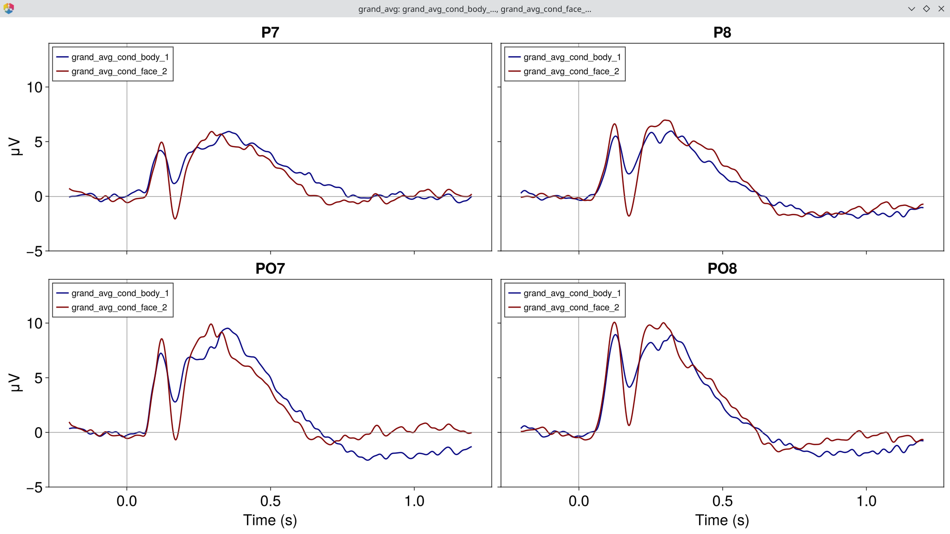

# Topography at the N170 peak (~170 ms)
EegFun.plot_topography(ga, interval_selection = EegFun.times(0.17))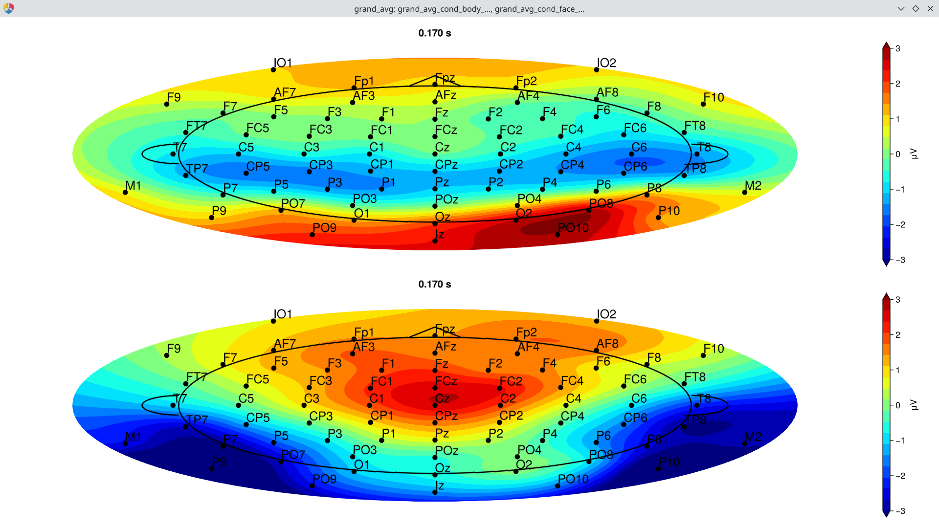

2.5 Difference Wave

Compute the difference wave (Face minus Body) to isolate the N170 face effect:

diff = EegFun.condition_difference(ga, [[2, 1]])

Plot the difference wave ERP at the N170 ROI:

EegFun.plot_erp(diff, baseline_interval = EegFun.times(-0.2, 0),
    channel_selection = EegFun.channels([:P7, :P8, :PO7, :PO8]), layout = :grid)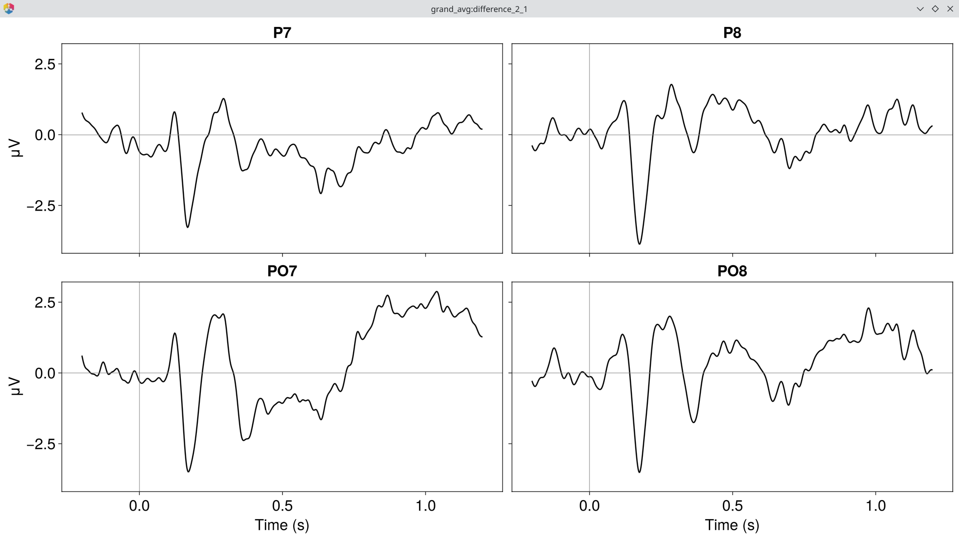

Topography of the difference wave at the N170 peak:

EegFun.plot_topography(diff, interval_selection = EegFun.times(0.17), ylim = (-3, 3))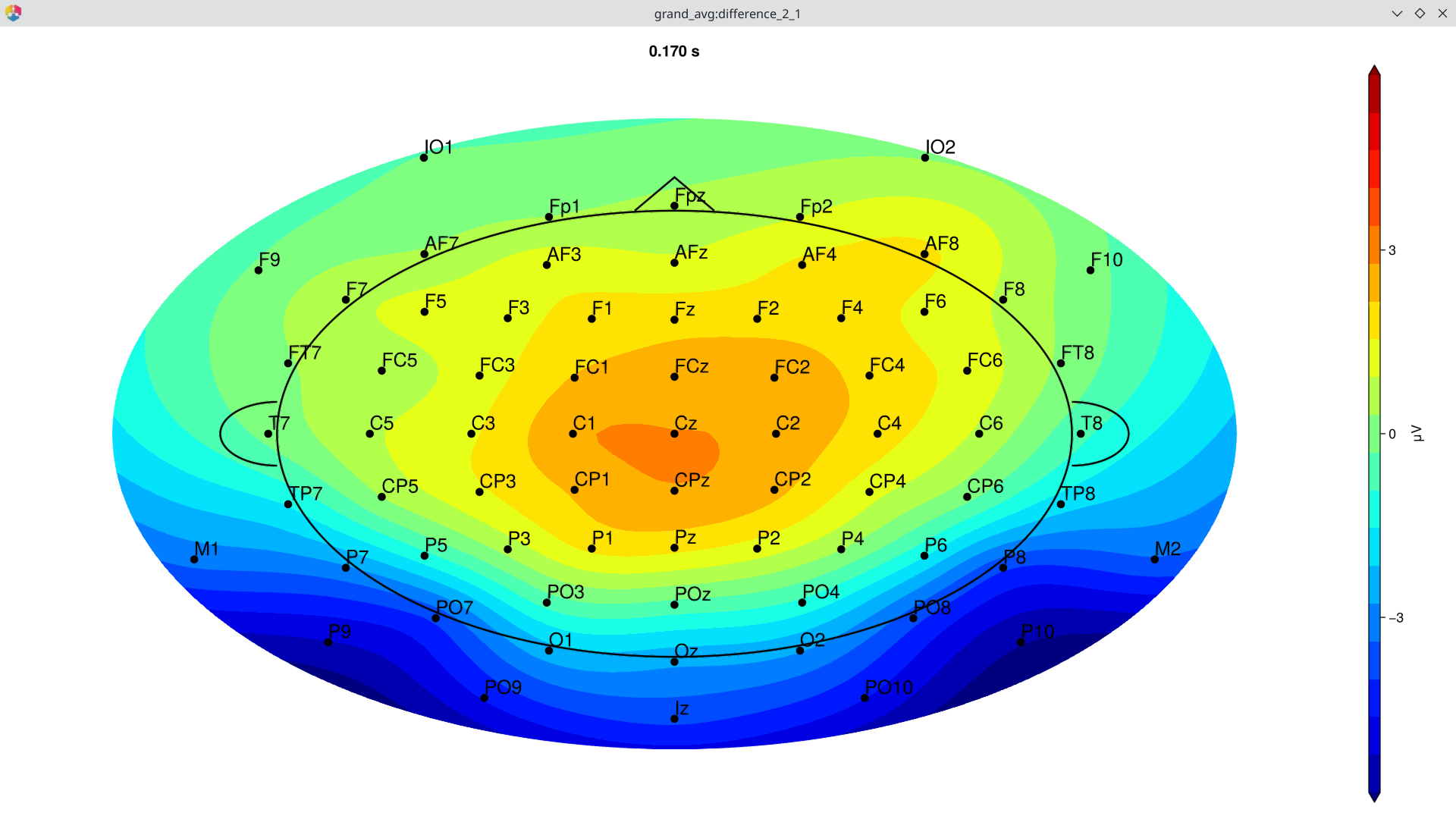

---

Part 3: Statistical Analysis

3.1 ERP Measurement GUI

Before extracting measurements in batch, use the interactive GUI to explore where and when to measure:

# Open the measurement GUI
EegFun.plot_erp_measurement_gui("./output_data/filtered_erps_good_lp_30hz/example1_erps_good.jld2")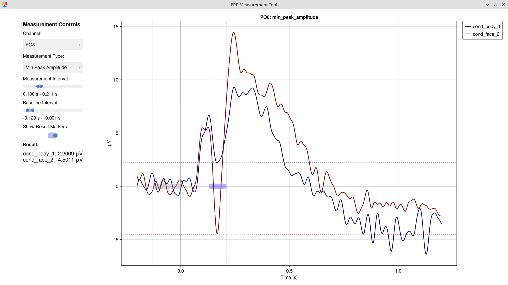

The GUI lets you select channels, time windows, and measurement types interactively to determine optimal parameters before running batch extraction. > > [!WARNING] The purpose of this step is to **verify** that your measurement window and type capture the component you intend to measure — not to search for channels or intervals where a difference happens to be significant. Choosing parameters based on observed effects inflates false-positive rates. Define your measurement strategy based on prior literature or orthogonal data, then use the GUI to confirm the settings look sensible. >

3.2 Extract ERP Measurements

Extract mean amplitude in the N170 window at posterior sites across all participants:

mean_amp = EegFun.erp_measurements(
    "erps_good",
    "mean_amplitude",
    input_dir = "./output_data/filtered_erps_good_lp_30hz/",
    condition_selection = EegFun.conditions([1, 2]),
    channel_selection = EegFun.channels([:P7, :P8, :PO7, :PO8]),
    analysis_interval = (0.15, 0.2),
    baseline_interval = (-0.2, 0.0),
)

# Result is an ErpMeasurementsResult containing a DataFrame
# Columns: participant, condition, P7, P8, PO7, PO8
mean_amp.data

3.3 Traditional Statistics

using AnovaFun
using Statistics

# Average across the 4 N170 ROI channels
mean_amp.data.roi .= mean(Matrix(mean_amp.data[:, [:P7, :P8, :PO7, :PO8]]), dims=2)

# --- Paired t-test: Body vs Face ---
result = paired_ttest(mean_amp.data, :roi, by = :condition)
result.t   # t-statistic
result.p   # p-value

3.4 Permutation-Based Statistics

Cluster-based permutation tests address the multiple comparisons problem across channels and time points:

# Prepare data for statistical testing
stat_data = EegFun.prepare_stats(
    "erps_good",
    :paired;
    input_dir = "./output_data/filtered_erps_good_lp_30hz/",
    condition_selection = EegFun.conditions([1, 2]),   # Body vs Face
    channel_selection = EegFun.channels(1:72),
    baseline_interval = EegFun.times((-0.2, 0.0)),
    analysis_interval = EegFun.times((0.0, 0.3)),
)

# Run cluster-based permutation test
result_perm = EegFun.permutation_test(
    stat_data,
    n_permutations = 1000,
    cluster_type = :spatiotemporal,
    show_progress = true,
)

# ERP waveforms with significance
fig = EegFun.plot_erp_stats(
    result_perm,
    channel_selection = EegFun.channels([:P7, :P8, :PO7, :PO8]),
    plot_erp = true,
    plot_significance = true,
    plot_se = true,
    layout = :grid,
    channel_plot_order = [:P7, :P8, :PO7, :PO8],
    xlim = (-0.2, 0.5),
    ylim = (-4, 12),
    legend_labels = ["Body", "Face"],
    xticks = -0.2:0.2:0.6,
    time_unit = :ms,
    legend_framevisible = false
)

---

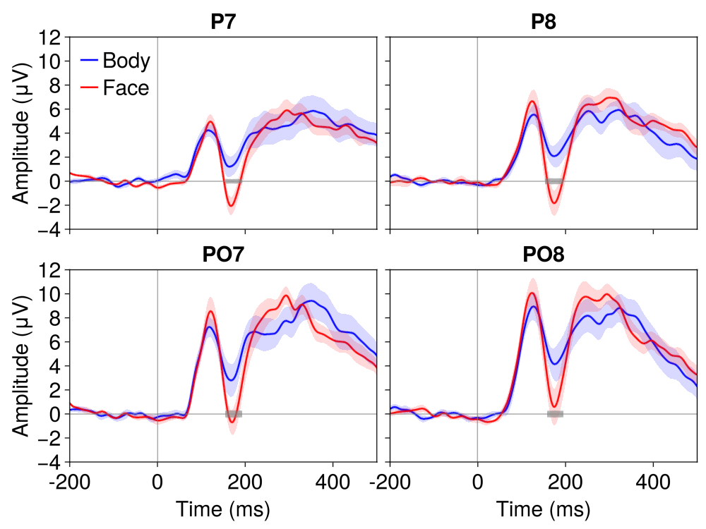
What to Look For

The N170 Face Effect

At posterior lateral channels (P7, P8, PO7, PO8):

• N170 component (~170 ms): Larger (more negative) for faces compared to body parts — reflects face-specific processing in the fusiform gyrus

• P1 component (~100 ms): May show a category difference, but typically smaller than the N170 effect

Lateralisation

The N170 is often right-lateralised for faces — compare P8/PO8 (right hemisphere) with P7/PO7 (left hemisphere) to check whether the face effect is stronger over the right hemisphere.

---

Further Reading

• Visual Attention (Posner Cueing) — Another worked example with cued attention

• Manual Preprocessing — Rationale behind each preprocessing step

• Batch Processing — preprocess() configuration

• Selection Patterns — The selector API

• Artifact Handling — Strategies for trial rescue

---

References

• Bentin, S., Allison, T., Puce, A., Perez, E., & McCarthy, G. (1996). Electrophysiological studies of face perception in humans. Journal of Cognitive Neuroscience, 8(6), 551–565. doi:10.1162/jocn.1996.8.6.551

---

The Whole Code

All code from this tutorial combined for easy copy-paste.

Part 1: Single Participant Exploration (click to expand)

using EegFun

# ── 1.1 Load Raw Data ──
dat = EegFun.read_raw_data("example1.bdf")
layout = EegFun.read_layout("biosemi72.csv")
dat = EegFun.create_eegfun_data(dat, layout)

# ── 1.2 Channel Layout and Neighbours ──
EegFun.plot_layout_2d(dat)
EegFun.get_neighbours_xy!(dat, 0.4)
EegFun.plot_layout_2d(dat, neighbours = true)
EegFun.viewer(dat.layout)
dat.layout.neighbours
EegFun.print_layout_neighbours(layout, "./neighbours.toml")

# ── 1.3 Inspect Triggers ──
EegFun.trigger_count(dat)
EegFun.plot_trigger_overview(dat)
EegFun.plot_trigger_timing(dat)

# ── 1.4 Browse the Raw Data ──
EegFun.viewer(dat)
EegFun.plot_databrowser(dat)
EegFun.highpass_filter!(dat, 0.1)
EegFun.rereference!(dat, :avg)
EegFun.plot_databrowser(dat)

# ── 1.5 Derive EOG Channels ──
EegFun.channel_difference!(dat,
    channel_selection1 = EegFun.channels([:Fp1, :Fp2]),
    channel_selection2 = EegFun.channels([:IO1, :IO2]),
    channel_out = :vEOG,
)
EegFun.channel_difference!(dat,
    channel_selection1 = EegFun.channels([:F9]),
    channel_selection2 = EegFun.channels([:F10]),
    channel_out = :hEOG,
)
EegFun.detect_eog_onsets!(dat, 50, :vEOG, :is_vEOG)
EegFun.detect_eog_onsets!(dat, 50, :hEOG, :is_hEOG)

# ── 1.6 Visualise Epoch Regions ──
EegFun.mark_epoch_intervals!(dat, [1, 2, 3, 5, 6], [-0.2, 1.2])
EegFun.plot_databrowser(dat)

# ── 1.7 Channel Quality and Extreme Values ──
cs = EegFun.channel_summary(dat)
EegFun.viewer(cs)
cs_epoch = EegFun.channel_summary(dat,
    sample_selection = EegFun.samples(:epoch_interval)
)
EegFun.viewer(cs)
EegFun.plot_channel_summary(cs, :range)
EegFun.plot_channel_summary(cs, [:range, :min, :max, :var])
EegFun.plot_channel_summary(cs_epoch, :range)
EegFun.is_extreme_value!(dat, 500)
EegFun.plot_databrowser(dat)

# ── 1.8 ICA ──
dat_ica = copy(dat)
EegFun.highpass_filter!(dat_ica, 1.0)
ica_result = EegFun.run_ica(dat_ica, sample_selection = EegFun.samples_not(:is_extreme_value_500))
EegFun.plot_topography(ica_result, component_selection = EegFun.components(1:10))
EegFun.plot_ica_component_activation(dat, ica_result)
EegFun.plot_databrowser(dat, ica_result)
component_artifacts, component_metrics = EegFun.identify_components(dat, ica_result,
    sample_selection = EegFun.samples_not(:is_extreme_value_500)
)
EegFun.plot_ica_component_activation(dat, ica_result, artifacts = component_artifacts)
all_removed = EegFun.get_all_ica_components(component_artifacts)
EegFun.remove_ica_components!(dat, ica_result,
    component_selection = EegFun.components(all_removed)
)
EegFun.plot_databrowser(dat)

# ── 1.9 Define Epoch Conditions ──
epoch_conditions = [
    EegFun.EpochCondition(name = "body", trigger_sequences = [[1], [2], [3]]),
    EegFun.EpochCondition(name = "face", trigger_sequences = [[5], [6]]),
]

# ── 1.10 Extract Epochs ──
epochs = EegFun.extract_epochs(dat, epoch_conditions, (-0.2, 1.2))
EegFun.baseline!(epochs, (-0.2, 0.0))
EegFun.plot_epochs(epochs, condition_selection = EegFun.conditions(1, 2), channel_selection = EegFun.channels(:P7))
EegFun.plot_epochs(epochs, layout = :grid)
EegFun.plot_epochs(epochs, condition_selection = EegFun.conditions(2), layout = :topo)

# ── 1.11 Reject Artifacts ──
rejection_info = EegFun.detect_bad_epochs_automatic(epochs, abs_criterion = 100.0, z_criterion = 0.0)
EegFun.plot_artifact_detection(epochs[1], rejection_info[1])
EegFun.plot_artifact_detection(epochs[2], rejection_info[2])
EegFun.channel_repairable!(rejection_info, epochs[1].layout)
EegFun.repair_artifacts!(epochs, rejection_info)
rejection_info2 = EegFun.detect_bad_epochs_automatic(epochs, abs_criterion = 100.0)
epochs_good = EegFun.reject_epochs(epochs, rejection_info2)

# ── 1.12 Average and Plot Single-Participant ERPs ──
erps = EegFun.average_epochs(epochs_good)
EegFun.plot_erp(erps, channel_selection = EegFun.channels([:P7, :P8, :PO7, :PO8]))
EegFun.plot_topography(erps, interval_selection = EegFun.times(0.17, 0.17))

Part 2: Batch Processing and Group Analysis (click to expand)

using EegFun

# ── 2.1 Batch Preprocessing ──
EegFun.preprocess("pipeline.toml")

# ── 2.2 Batch Filter ERPs ──
EegFun.lowpass_filter("erps_good", 30, input_dir = "./output_data")

# ── 2.3 Grand Average ──
EegFun.grand_average("erps_good",
    input_dir = "./output_data/filtered_erps_good_lp_30hz"
)

# ── 2.4 Publication-Quality Plots ──
ga = EegFun.read_data(
    "./output_data/filtered_erps_good_lp_30hz/grand_average_erps_good/grand_average_erps_good.jld2"
)
EegFun.plot_erp(ga, baseline_interval = EegFun.times(-0.2, 0),
    channel_selection = EegFun.channels([:P7, :P8, :PO7, :PO8]), layout = :grid, ylim = (-5, 15))
EegFun.plot_topography(ga, interval_selection = EegFun.times(0.17))

# ── 2.5 Difference Wave ──
diff = EegFun.condition_difference(ga, [[2, 1]])
EegFun.plot_erp(diff, baseline_interval = EegFun.times(-0.2, 0),
    channel_selection = EegFun.channels([:P7, :P8, :PO7, :PO8]), layout = :grid)
EegFun.plot_topography(diff, interval_selection = EegFun.times(0.17), ylim = (-3, 3))

Part 3: Statistical Analysis (click to expand)

using EegFun, AnovaFun, Statistics

# ── 3.1 ERP Measurement GUI ──
EegFun.plot_erp_measurement_gui("./output_data/filtered_erps_good_lp_30hz/example1_erps_good.jld2")

# ── 3.2 Extract ERP Measurements ──
mean_amp = EegFun.erp_measurements(
    "erps_good",
    "mean_amplitude",
    input_dir = "./output_data/filtered_erps_good_lp_30hz/",
    condition_selection = EegFun.conditions([1, 2]),
    channel_selection = EegFun.channels([:P7, :P8, :PO7, :PO8]),
    analysis_interval = (0.15, 0.2),
    baseline_interval = (-0.2, 0.0),
)

# ── 3.3 Traditional Statistics ──
mean_amp.data.roi .= mean(Matrix(mean_amp.data[:, [:P7, :P8, :PO7, :PO8]]), dims=2)
result = paired_ttest(mean_amp.data, :roi, by = :condition)
result.t   # t-statistic
result.p   # p-value

# ── 3.4 Permutation-Based Statistics ──
stat_data = EegFun.prepare_stats(
    "erps_good",
    :paired;
    input_dir = "./output_data/filtered_erps_good_lp_30hz/",
    condition_selection = EegFun.conditions([1, 2]),
    channel_selection = EegFun.channels(1:72),
    baseline_interval = EegFun.times((-0.2, 0.0)),
    analysis_interval = EegFun.times((0.0, 0.3)),
)

result_perm = EegFun.permutation_test(
    stat_data,
    n_permutations = 1000,
    cluster_type = :spatiotemporal,
    show_progress = true,
)

# ERP waveforms with significance
fig = EegFun.plot_erp_stats(
    result_perm,
    channel_selection = EegFun.channels([:P7, :P8, :PO7, :PO8]),
    plot_erp = true,
    plot_significance = true,
    plot_se = true,
    layout = :grid,
    channel_plot_order = [:P7, :P8, :PO7, :PO8],
    xlim = (-0.2, 0.5),
    ylim = (-4, 12),
    legend_labels = ["Body", "Face"],
    xticks = -0.2:0.2:0.6,
    time_unit = :ms,
    legend_framevisible = false
)