Plot GUI
The Plot GUI is a quick-access point for interactively exploring your EEG data. Launch it with a single command and use it to inspect any raw EEG file or saved JLD2 data file — or an entire batch of files at once using filename patterns.
Launching the GUI
using EegFun
EegFun.plot_gui()
A window opens with three columns allowing file selection, plot selection, and plot setting type controls.
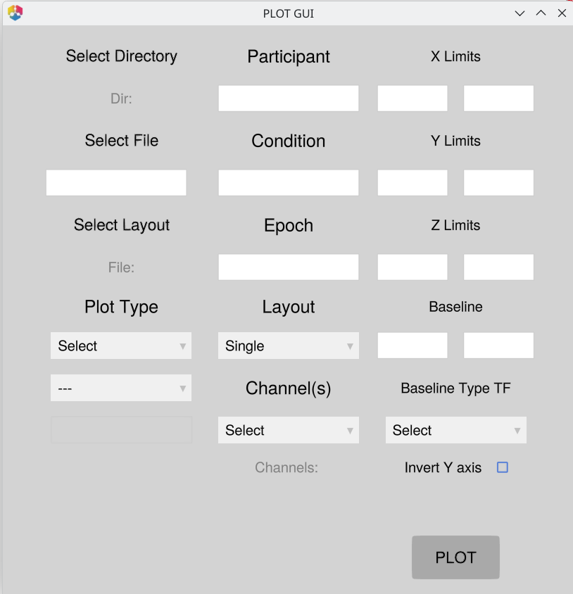
GUI Layout
The window is divided into three columns.
Column 1 — File & Plot Selection
| Control | Description |
|---|---|
| Select Directory | Sets the working directory used for batch file discovery |
| (directory label) | Shows the currently selected directory path |
| Select File | Opens a file picker to choose a .jld2 or raw EEG file |
| (file / pattern box) | Type a filename, full path, or batch pattern directly |
| Select Layout | Opens a file picker to load an electrode layout (.csv) |
| (layout label) | Shows the currently loaded layout filename |
| Plot Type | Dropdown — direct plots or category submenus (ICA >, ERP Analysis >, Diagnostic Plots >) |
| (submenu) | Appears when a category is selected; choose the specific plot type |
| (components box) | Active only for ICA plots — enter component numbers to plot |
Column 2 — Data Filters
| Control | Description |
|---|---|
| Participant | Space/comma-separated integers or ranges (e.g. 1 2 3 or 1:10) |
| Condition | Condition numbers to include; blank = all |
| Epoch | Epoch numbers to include; blank = all |
| Layout | Plot layout: Single, Single Avg, Grid, Topo |
| Channel(s) | Multi-select menu (populated when a layout is loaded) |
| (selected label) | Shows the currently selected channels |
Column 3 — Axis Settings
| Control | Description |
|---|---|
| X Limits | Min / max for the time axis |
| Y Limits | Min / max for the amplitude axis |
| Z Limits | Min / max for the colour axis (TF and ERP Image) |
| Baseline | Start / end times in seconds for baseline correction |
| Baseline Type TF | Baseline normalisation method for Time-Frequency plots |
| Invert Y axis | Checkbox — flips the Y axis (ERP, Epochs, ERP Image) |
| PLOT | Triggers the selected plot |
Step-by-Step: Plotting a Single File
1. Pick a directory
Click Select Directory to set the working directory.
For batch mode (pattern input) this is essential — it tells the GUI where to search for matching files. If left unset, the GUI falls back to pwd(), which is the directory Julia was launched from and is rarely where your data lives.
For single-file mode (Select File picks a full path) the directory is not required.
2. Select a file
Either:
Click Select File and navigate to a
.jld2or raw EEG file, orType the filename directly into the text box.
The text box accepts full paths, relative paths, or just a filename if the directory is already set.
3. Choose a plot type
Click the Plot Type dropdown and select one of the direct plot types:
| Selection | Produces |
|---|---|
| Data Browser | Interactive scrollable signal browser |
| Epochs | Epoch-level waveform viewer |
| ERP | ERP waveforms |
| ERP Image | Heatmap of individual epochs |
| Topography | Scalp topographic map |
| Time-Frequency | Time-frequency power plot |
For more specialised plots, select a category to reveal a submenu:
| Category | Submenu options |
|---|---|
| ICA > | Components (topographies), Activation (time-course) |
| ERP Analysis > | ERP GUI |
| Diagnostic Plots > | Channel Summary, Layout View |
4. Configure controls (optional)
All controls are optional — leave them blank to use sensible defaults.
X / Y / Z limits — Enter a min and max value in the paired text boxes to constrain the plotted time range (X), amplitude scale (Y), or colour scale (Z). Both boxes must be filled for the limit to apply.
Baseline — Enter start and end times in seconds (e.g. -0.2 and 0.0) and choose a correction method from the dropdown.
Channels — If a layout file is loaded, pick one or more channels from the Channels menu. Click Select to clear the selection.
Layout — Choose how channels are arranged:
Single — all selected channels overlaid on one axis
Grid — one axis per channel in a grid
Topo — channels positioned according to their electrode locations
Single Avg — channels averaged together before plotting
Invert Y axis — Tick this checkbox to plot positive deflections downward, matching the neurophysiology convention used in some ERP labs. Applies to ERP, Epochs, and ERP Image plots.
5. Click Plot
Click the Plot button. The plot opens in a new window.
Batch Mode (Pattern Input)
Instead of a single filename, type a filename pattern into the file box. EegFun will discover all matching .jld2 files in the selected directory and plot them one after another.
# Example: type this into the file box
erps_good
This matches any file containing erps_good in the directory (e.g. 01_erps_good.jld2, 02_erps_good.jld2, …).
Filtering by participant
Enter participant numbers in the Participant box (space- or comma-separated integers, or ranges):
1 2 3         # participants 1, 2, and 3
1:10          # participants 1 through 10
1 3 5:8       # mixed
If the box is empty, all matching participants are plotted.
Filtering by condition
Enter condition numbers in the Condition box using the same syntax. Leave blank to plot all conditions.
If you enter a participant ID that does not exist in the discovered files, the GUI will warn you and list the available IDs before plotting.
ICA Plots
Select ICA > from the Plot Type dropdown to see two options.
Components — Plots the ICA component topographies. The file must be an InfoIca .jld2 produced by run_ica().
Activation — Plots the ICA component activation time-courses. The GUI automatically locates the original EEG source file from the path stored inside the InfoIca object. If the source file is a raw format (.bdf, .set, .vhdr), a 0.1 Hz high-pass filter and average rereference are applied automatically before plotting.
Use the Components text box to restrict which components are shown:
1:10          # first ten components
1 3 5         # specific components
              # (blank = all components)
Layout File
Some plot types (Data Browser with a raw .bdf file, Layout View) require an electrode layout. Click Select Layout to load a .csv layout file. The channel list in the Channels menu is then populated from the layout.
Tips
Data Browser with a
.bdffile requires a layout to be loaded.Z limits apply only to Time-Frequency and ERP Image plots (colour axis).
Baseline fields apply to ERP and Time-Frequency plots.
The GUI state is preserved between plots — change one setting at a time to compare results.
If a plot fails, a brief warning appears in the Julia REPL. The GUI remains open and usable.
Next Steps
Preprocessing your data — Manual Preprocessing or Batch Processing to produce clean epochs and ERPs to explore in the GUI
Layouts — Layouts and Neighbours for loading the layout file required by topographic and data browser plots
Artifact review — Artifact Handling for the
detect_bad_epochs_interactiveGUI workflow