
Simulate ERP — Signal Averaging Demo
Interactive ERP simulator for teaching how trial averaging extracts signals from noise.
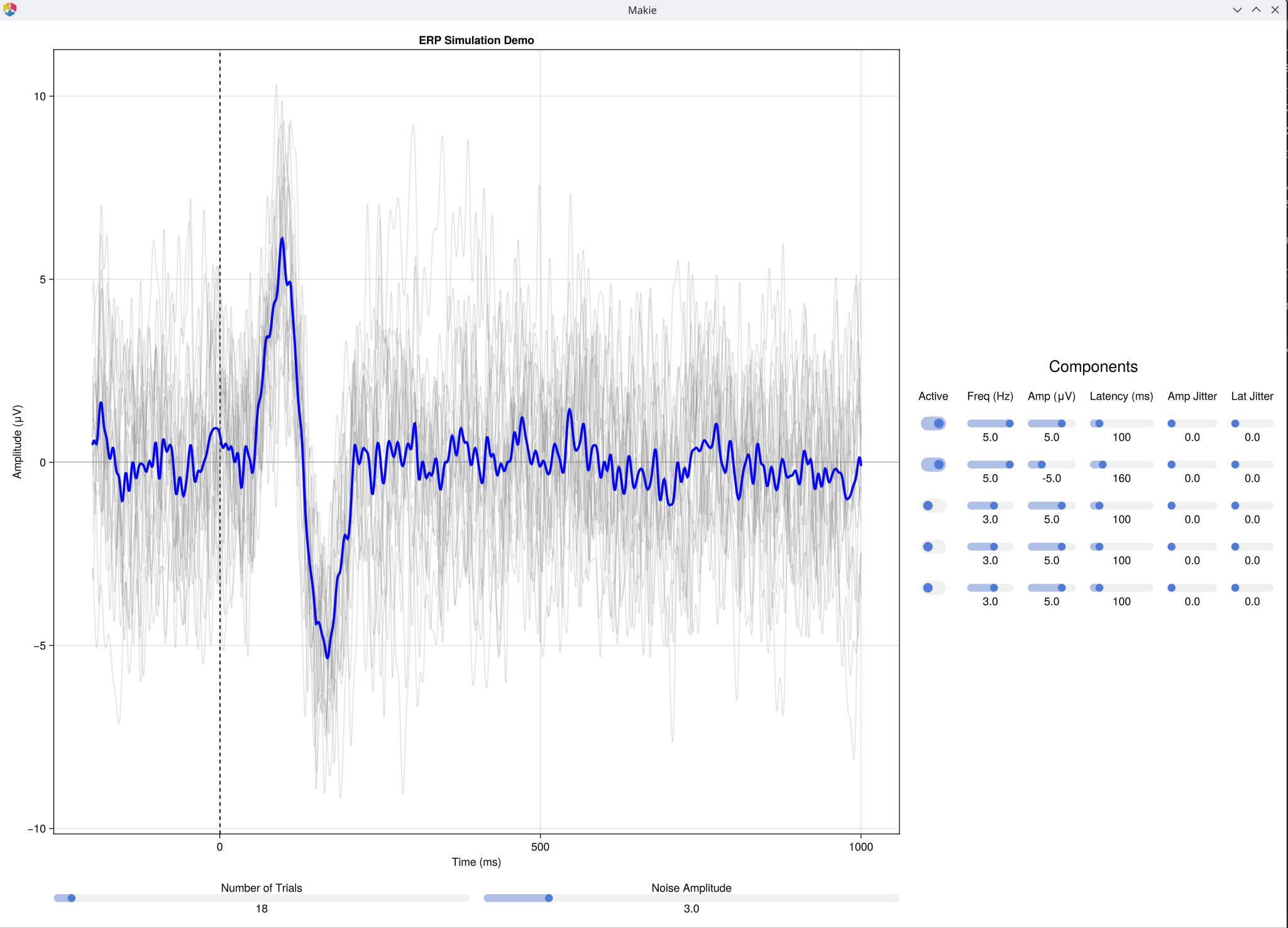
What it shows
| Element | Description |
|---|---|
| Grey lines | Individual simulated EEG trials with realistic 1/f background noise |
| Blue line | Trial-average ERP — clarifies as more trials are added |
| Components | Up to 5 independent ERP components, each shaped as a single cosine lobe (the central peak of a cosine wave, masked to ±π/2) to produce a smooth, bell-like waveform |
The core insight: The signal-to-noise ratio of the ERP average scales with √N (where N is the number of trials). Doubling the number of trials improves SNR by ~41%; to halve the noise, you need 4× as many trials.
The background noise uses a realistic human EEG power spectrum (1/f structure), not white noise — so individual trials look like real EEG epochs rather than random static.
This demo builds directly on Signal Example 2: the ERP waveform you see in the average is a real-world instance of multiple frequency components summing together, now embedded in realistic noise.
Things to Try
Start with 1 trial and a single active component — the ERP equals the single trial.
Add noise and increase trials to watch the ERP "emerge" from the background activity.
Activate a second component at a different latency to show how components superpose — and try setting one to a negative amplitude to model typical ERP polarities (N1 negative, P3 positive).
Introduce latency jitter to show how trial-to-trial variability smears and attenuates the average — a key confound in real ERP research.
Introduce amplitude jitter to show how variability in peak amplitude scales the average downward.
Controls
Each component has its own row of controls in the right panel.
| Control | Range | Description |
|---|---|---|
| Number of Trials | 1–500 | Trials to average |
| Noise Amplitude | 0–20 | Background 1/f EEG noise level |
| Active toggle (×5) | on/off | Enable or disable each component |
| Freq (×5) | 0.1–5.0 Hz | Component shape (cosine frequency) |
| Amp (×5) | −10 to 10 μV | Peak amplitude (negative = typical N-wave polarity) |
| Latency (×5) | 0–1000 ms (steps: 10 ms) | Peak latency |
| Amp Jitter (×5) | 0–20 (Gaussian SD) | Trial-to-trial amplitude variability |
| Lat Jitter (×5) | 0–50 ms (Gaussian SD) | Trial-to-trial latency variability |
See Also
Luck, S. J. (2014). An Introduction to the Event-Related Potential Technique (2nd ed.). MIT Press. — Chapter 8 (averaging and signal-to-noise ratio)
Signal Example — Sampling — Nyquist theorem and signal reconstruction
Signal Example — Composition — signal composition and filtering
Simulate Decoding — multivariate pattern classification on synthetic EEG
Code
using EegFun
EegFun.simulate_erp()