Signal Example — Signal Composition & Filtering
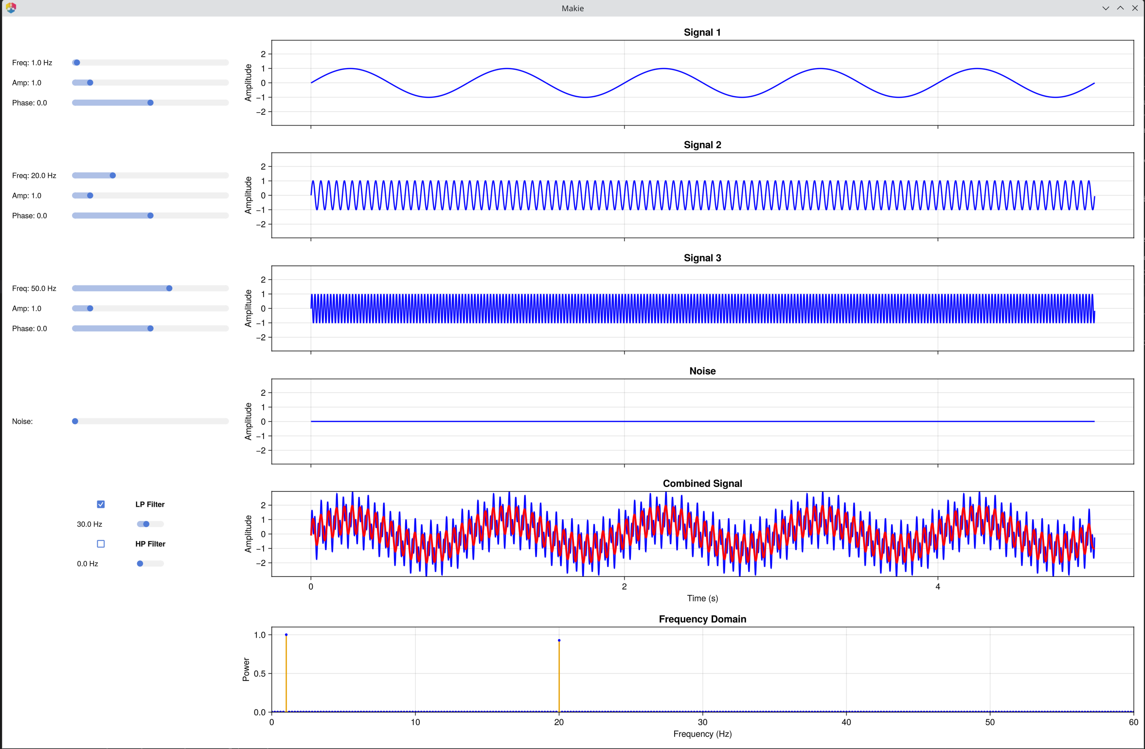
Interactive multi-signal composer demonstrating how complex waveforms are built from simple sine waves, how noise affects a signal, and how filters shape the frequency content.
What it shows
| Row | Plot | Description |
|---|---|---|
| 1–3 | Signal 1–3 | Individual sine waves (y-axes linked for direct amplitude comparison) |
| 4 | Noise | Additive Gaussian noise |
| 5 | Combined Signal | Sum of all signals plus noise; a red overlay shows the filtered version when a filter is active |
| 6 | Frequency Domain | Power spectrum (amplitude²) of the combined signal (or the filtered signal when a filter is active) |
The x-axes of all five time-domain plots are linked — panning or zooming one panel updates all of them simultaneously. The y-axes of Signal 1–3 are also linked, so amplitude changes remain visually comparable across all three.
Things to Try
Start with a single signal (Amp > 0 for Signal 1 only) and observe its clean spectral peak.
Add a second frequency to show how signals superpose in the time domain and produce two peaks in the spectrum.
Increase noise and watch the spectral floor rise until the signal peaks are buried — a direct illustration of the signal-to-noise problem in EEG.
Enable the LP filter and sweep its cutoff to demonstrate how filtering removes high-frequency content while preserving low-frequency structure.
Enable the HP filter and set a low cutoff (e.g. 0.1–1 Hz) to show how slow drifts are removed — a common preprocessing step in EEG.
Controls
Each signal row has its own frequency, amplitude, and phase controls in the left panel.
| Control | Range | Description |
|---|---|---|
| Freq (×3) | 0–80 Hz | Frequency of each sine wave |
| Amp (×3) | 0–10 | Amplitude of each sine wave |
| Phase (×3) | −π to π | Phase offset of each sine wave |
| Noise | 0–2 | Standard deviation of additive Gaussian noise |
| ☐ LP Filter | 0–100 Hz | Low-pass filter cutoff |
| ☐ HP Filter | 0–2 Hz | High-pass filter cutoff (typical EEG values: 0.1–1 Hz) |
See Also
Luck, S. J. (2014). An Introduction to the Event-Related Potential Technique (2nd ed.). MIT Press. — Chapter 1 (Figure 1.6)
Signal Example — Sampling — Nyquist theorem and signal reconstruction
Signal Example — Dot Product — how the DFT detects individual frequencies
Signal Example — Spectrum — the full FFT power spectrum
Code
using EegFun
EegFun.signal_example_composition()