Signal Example — Sampling & Reconstruction

Interactive demonstration of the Nyquist–Shannon sampling theorem.

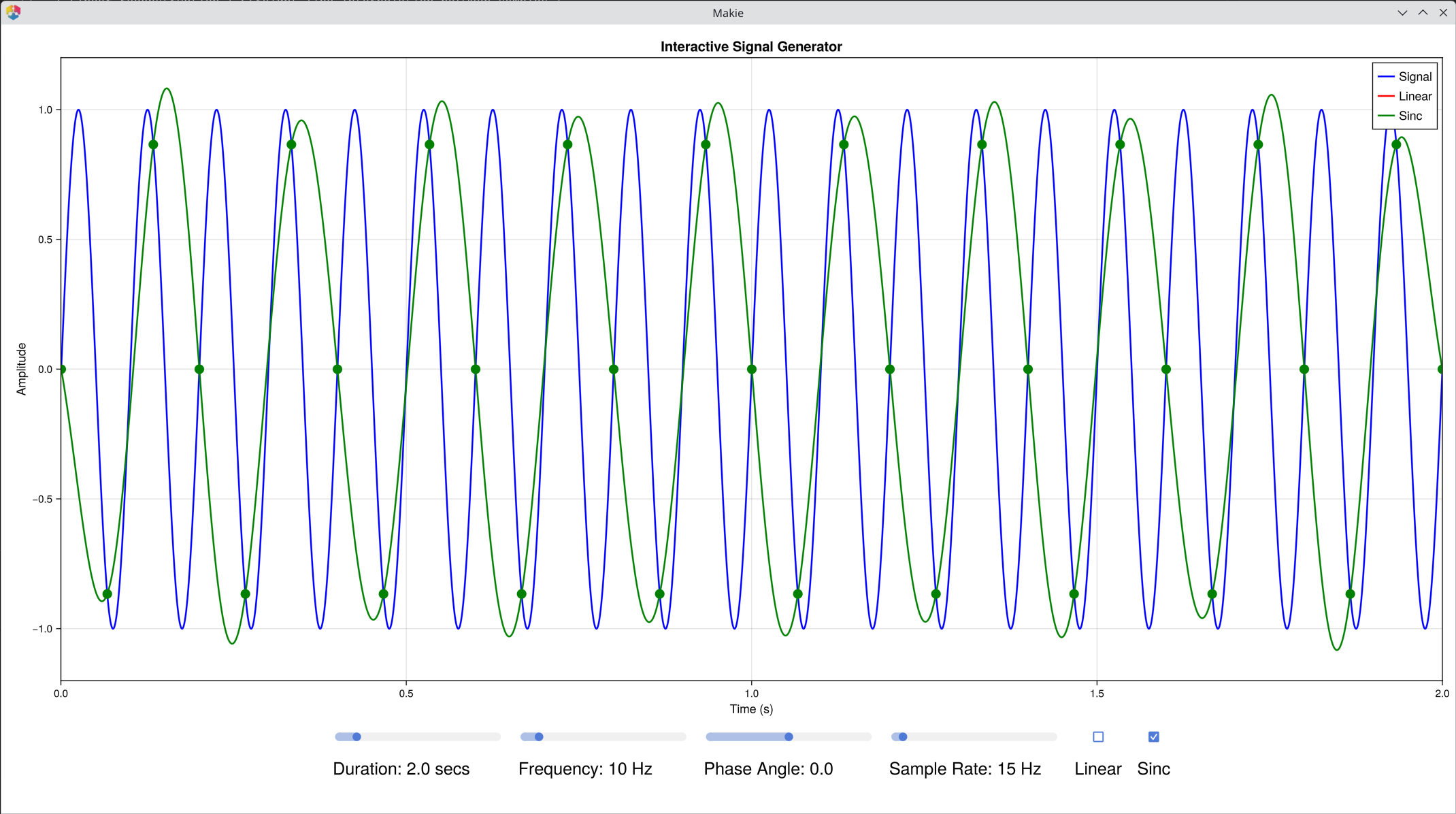
This demo shows how sampling rate affects the reconstruction of a sine wave.

What it shows

Feature	Description
Original signal	A "continuous" sine wave at the chosen frequency
Sampled points	The discrete samples taken at the chosen sampling rate
Linear reconstruction	Straight-line interpolation between samples
Sinc reconstruction	Whittaker–Shannon (ideal) interpolation

Linear reconstruction connects adjacent samples with straight lines. It is simple but introduces distortion — particularly at low sampling rates relative to the signal frequency.

Sinc reconstruction uses the Whittaker–Shannon interpolation formula to reconstruct the signal exactly (within the Nyquist limit).

When the sampling rate falls below twice the signal frequency, the signal cannot be recovered: the sampled waveform appears at the wrong frequency — a phenomenon known as aliasing. Modern EEG systems typically sample at 256–2048 Hz, which is far above the Nyquist limit for brain signals of interest (usually < 100 Hz), ensuring faithful digitisation.

Things to Try

• Start with a sampling rate well above Nyquist (e.g. 10× the signal frequency) and observe that both methods agree with the original signal.

• Gradually reduce the sampling rate toward and then below the Nyquist limit (~2× the signal frequency) to show reconstruction breakdown and aliasing.

• Enable both reconstructions simultaneously to highlight the superiority of sinc interpolation near the Nyquist limit.

Controls

Control	Range	Description
Duration	1–10 s	Length of the displayed signal
Signal Frequency	1–100 Hz	Frequency of the underlying sine wave
Phase Angle	−π to π	Phase offset of the sine wave
Sampling Rate	1–300 Hz	Number of samples per second
☐ Linear	—	Toggle linear interpolation overlay
☐ Sinc	—	Toggle sinc reconstruction overlay

See Also

• Luck, S. J. (2014). An Introduction to the Event-Related Potential Technique (2nd ed.). MIT Press. — Chapter 5 (Section: Amplifying, Filtering, and Digitizing the Signal, Figure 5.7)

• Sinc Interpolation for Signal Reconstruction (Wolfram Demonstrations)

• Signal Example — Composition — multi-signal composition and filtering

• Signal Example — Dot Product — how the DFT detects frequencies

• Signal Example — Spectrum — the full FFT power spectrum

Code

using EegFun
EegFun.signal_example_sampling()