Signal Example — Time-Frequency Analysis
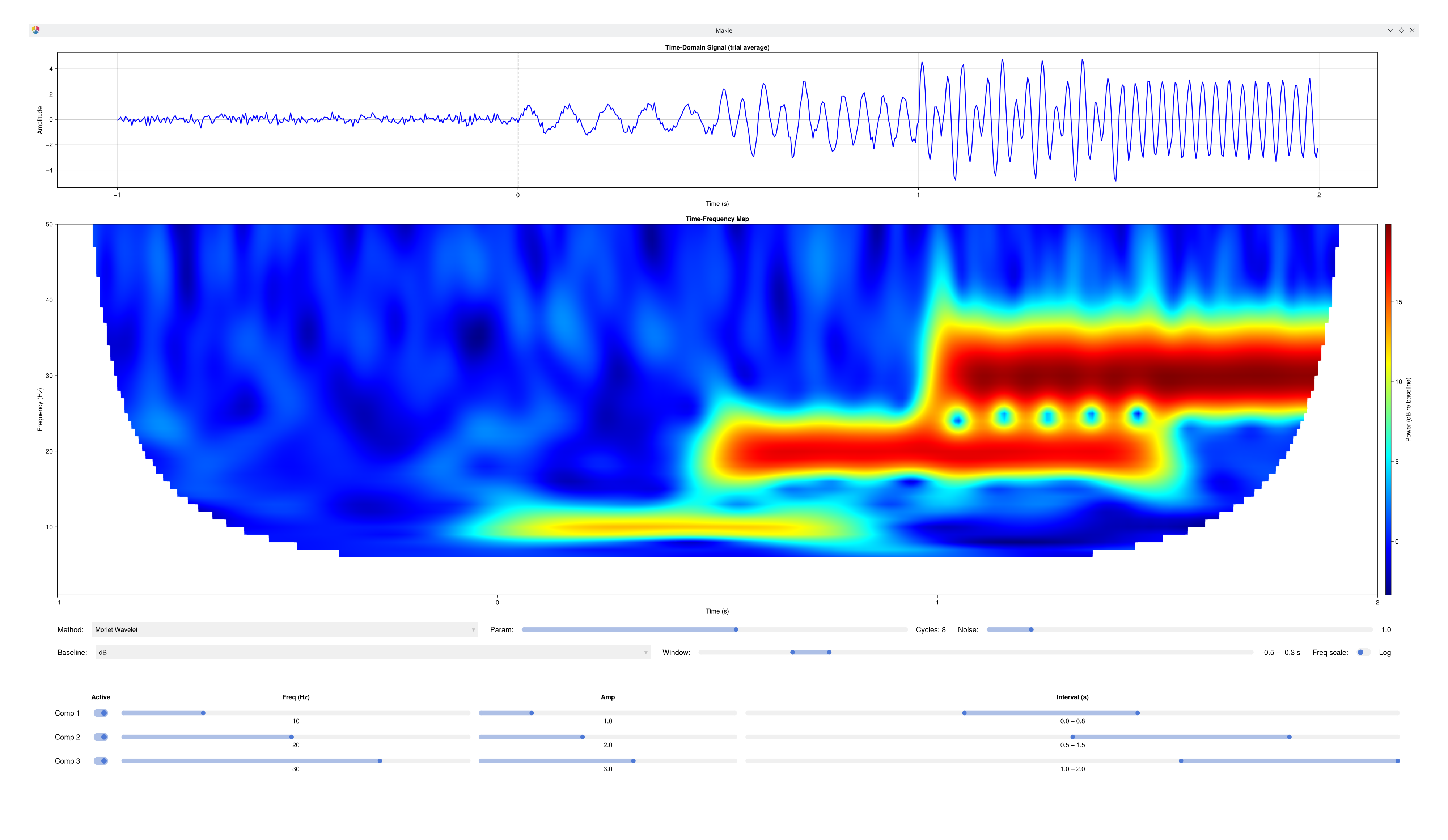
Interactive demo comparing three time-frequency analysis methods on a synthetic multi-component signal, with controls for baseline normalization and frequency-axis scaling.
What it shows
| Row | Plot | Description |
|---|---|---|
| 1 | Time Domain | Synthetic signal averaged across 20 trials. Dashed line = t = 0. |
| 2 | Time-Frequency Map | Power heatmap from the selected method, optionally baseline-corrected. |
Up to three independent frequency components can be active simultaneously, each with its own onset–offset interval. This lets you directly compare how each method handles multiple overlapping signals with different frequencies and timings.
The Core Idea: Heisenberg's Uncertainty Principle
You cannot have perfect time and frequency resolution simultaneously — narrowing one always blurs the other. Every TF method is a choice about where to make that trade-off.
| Method | Window | Resolution trade-off |
|---|---|---|
| Morlet Wavelet | Gaussian, adaptive | At 10 Hz: wide window → sharp frequency, poor time. At 40 Hz: narrow window → sharp time, blurry frequency. The window scales automatically with frequency. |
| STFT (Hanning) | Hanning, fixed | Same window length for all frequencies → uniform resolution. 233 ms window gives ~4 Hz frequency resolution at every band. |
| Multitaper (DPSS) | Slepian tapers, adaptive | Like Morlet but averages across multiple orthogonal tapers → lower variance estimates at the cost of slight frequency smoothing. |
Cohen (2014), Ch. 12–13 — Morlet Wavelets and Wavelet Convolution Cohen (2014), Ch. 15 — Short-time FFT Cohen (2014), Ch. 16 — Multitaper
Baseline Normalization
Raw TF power cannot be compared across methods, frequencies, or participants because absolute power varies with electrode impedance, distance from the source, and method-specific scaling. Baseline normalization expresses power relative to a reference period (typically pre-stimulus).
| Method | Formula | Range | When to use |
|---|---|---|---|
| None | raw power | unbounded | Comparing absolute power (rarely appropriate) |
| dB | 10·log₁₀(P / BL) | unbounded, 0 at baseline | Most robust for EEG — log compression handles large dynamic range |
| % Change | 100·(P − BL) / BL | unbounded, 0 at baseline | Intuitively interpretable scale |
| Z-score | (P − BL_mean) / BL_std | z-units | Group-level comparison; requires stable baseline std |
| Relative | P / BL_mean | ratio, 1 at baseline | Clean background; can't compare across frequencies |
| Rel. Change | (P − BL) / BL | ratio, 0 at baseline | Like % Change without the ×100 |
| Norm. Change | (P − BL) / (P + BL) | −1 to +1 | Sensitive to small fluctuations in low-SNR regions |
| Absolute | P − BL | same units as power | Rarely used; frequency-dependent bias |
The baseline window defaults to −1.0 – 0.0 s (pre-stimulus). Move it with the IntervalSlider — it can be placed anywhere in the epoch.
Cohen (2014), Ch. 18 — Time-Frequency Power and Baseline Normalizations
Things to Try
1. The resolution trade-off (Morlet) Enable Comp 1 (10 Hz, 0.0 – 0.8 s), baseline = dB. Sweep the Param slider from 3 to 12 cycles: watch the blob grow narrow in frequency but wide in time at high cycles, and vice versa. This is Heisenberg in action.
2. Morlet vs. STFT on the same signal Add Comp 3 (40 Hz, 1.0 – 2.0 s). Switch between Morlet and STFT with Param = 7. Notice:
STFT: all three component blobs are the same rectangular shape regardless of frequency.
Morlet: the 10 Hz blob is wider in time, the 40 Hz blob is narrower — because the window adapts.
3. STFT onset artifact Set Param to 3 (short window = 100 ms), enable only Comp 1, set baseline = None. Switch to STFT. The "flame" pattern at onset is real physics: as the fixed Hanning window slides past the signal's hard edge at t = 0, it captures successive phases of the 10 Hz oscillation, producing structured amplitude modulation across the transition. Switch to Morlet — the Gaussian taper handles the onset far more gracefully.
4. Multitaper variance reduction Enable all three components with a moderate noise (Noise = 2.0). Toggle rapidly between Morlet and Multitaper: the Multitaper map is smoother because it averages independent spectral estimates from multiple orthogonal Slepian tapers, reducing random variance without introducing the bias that additional smoothing would.
5. Baseline normalization sensitivity Set three components active and baseline = dB. Sweep the baseline window across the stimulus period: you can clearly see the baseline reference contaminating the normalization when signal is included. Move it back to pre-stimulus only to see clean dB increases.
6. Log frequency axis Enable the Log toggle. Low frequencies are spread out — revealing fine structure in the 1–10 Hz range — while high frequencies compress. This matches the 1/f power distribution of real EEG.
Controls
| Control | Range | Description |
|---|---|---|
| Method | Morlet / STFT / Multitaper | TF decomposition method |
| Param | 3–12 | Cycles (Morlet/Multitaper) or window ≈ N/30 Hz in ms (STFT) |
| Noise | 0.5–5 | Amplitude of additive white noise per trial |
| Baseline | None / dB / % Change / … | Baseline correction method (all EegFun tf_baseline types) |
| Window | −1.0–2.0 s | Baseline time window (IntervalSlider) |
| Freq scale | Linear / Log | Toggle log₁₀ y-axis on the TF map |
| ☐ Comp 1/2/3 | on/off | Enable/disable each component |
| Freq (×3) | 1–40 Hz | Component frequency |
| Amp (×3) | 0–5 | Component amplitude |
| Interval (×3) | −1.0–2.0 s | Component onset–offset window (IntervalSlider) |
See Also
Cohen, M. X. (2014). Analyzing Neural Time Series Data. MIT Press.
Section III: Frequency and Time-Frequency Domains Analyses
Signal Example — Sampling — Nyquist theorem and sampling
Signal Example — Composition — signal composition and filtering
Signal Example — Spectrum — the full FFT power spectrum
Signal Example — Convolution — sliding kernels including Morlet wavelets
Code
using EegFun
EegFun.signal_example_tf()