Signal Example — Convolution

Interactive demo showing discrete convolution by sliding a kernel across a signal, with three kernel types including a Morlet wavelet to bridge filtering and time-frequency analysis.

What it shows

Row	Plot	Description
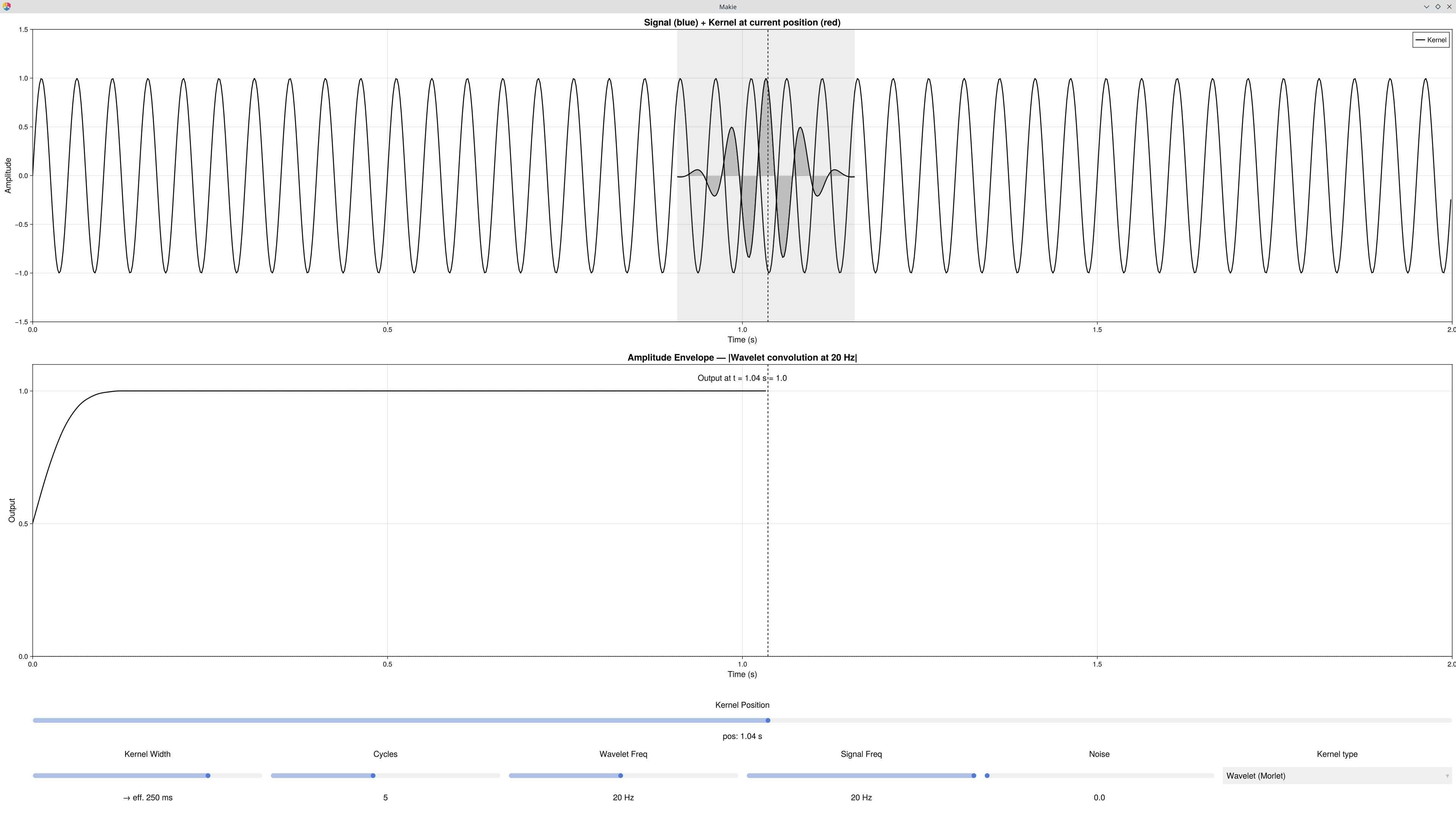
1	Signal + Kernel	The input signal with the kernel overlaid at the current position — the shaded band marks the overlap region.
2	Output	The convolution result accumulated up to the current kernel position. For the Wavelet kernel, this is the amplitude envelope.

Key Concept

Convolution computes, at each time point t, the weighted sum of the signal under the kernel:

Gaussian: smooth low-pass filter — noise suppressed, slow waves preserved.

Boxcar: running average — same idea but with sharper edges in frequency.

Wavelet (Morlet): Gaussian × cos(2πfτ) — the kernel is frequency-selective. The output is the amplitude envelope: how much of Wavelet Freq is present at each time point. This is one row of a time-frequency spectrogram.

Controls

Control	Applies to	Description
Kernel Position	All	Scrub the kernel across the signal — output builds up as you drag right
Kernel Width	Gaussian / Boxcar	Total span of the kernel (label updates to "→ eff. X ms" in Wavelet mode)
Cycles	Wavelet	Number of oscillations in the kernel — more cycles = better frequency resolution, worse time resolution
Wavelet Freq	Wavelet	The target frequency to detect
Signal Freq	All	Frequency of the input signal
Noise	All	Additive Gaussian noise
Kernel type	All	Switch between Gaussian, Boxcar, Wavelet (Morlet)

Things to Try

1. Low-pass filtering: Gaussian kernel, drag position to end — output is a smoother version of the noisy input.

2. Kernel width effect: Gaussian, widen the kernel → noise disappears, but the sine is also attenuated as the kernel begins to span whole cycles.

3. Switch to Wavelet Freq = Signal Freq → amplitude envelope is near 1.0 (frequency detected).

4. Mismatch frequencies (e.g. Wavelet = 8 Hz, Signal = 4 Hz) → envelope near 0.

5. Cycles tradeoff: with two nearby signal frequencies, fewer cycles blurs them together; more cycles separates them.

6. Link to Gaussian: set Kernel Width = value shown in "→ eff. X ms" label, then switch kernel type — you will see the same Gaussian envelope.

See Also

• Signal Example — Composition — building signals from sine waves

• Signal Example — Dot Product — the core dot product mechanism

• Signal Example — Spectrum — the full FFT spectrum

• Signal Example — Time-Frequency — running Morlet convolution at every frequency

• Cohen, M. X. (2014). Analyzing Neural Time Series Data. MIT Press. — Chapter 11/12

Code

using EegFun
EegFun.signal_example_convolution()