Simulate Decoding — MVPA Playground
Interactive demo showing time-resolved multivariate pattern classification (MVPA/decoding) on synthetic EEG data.
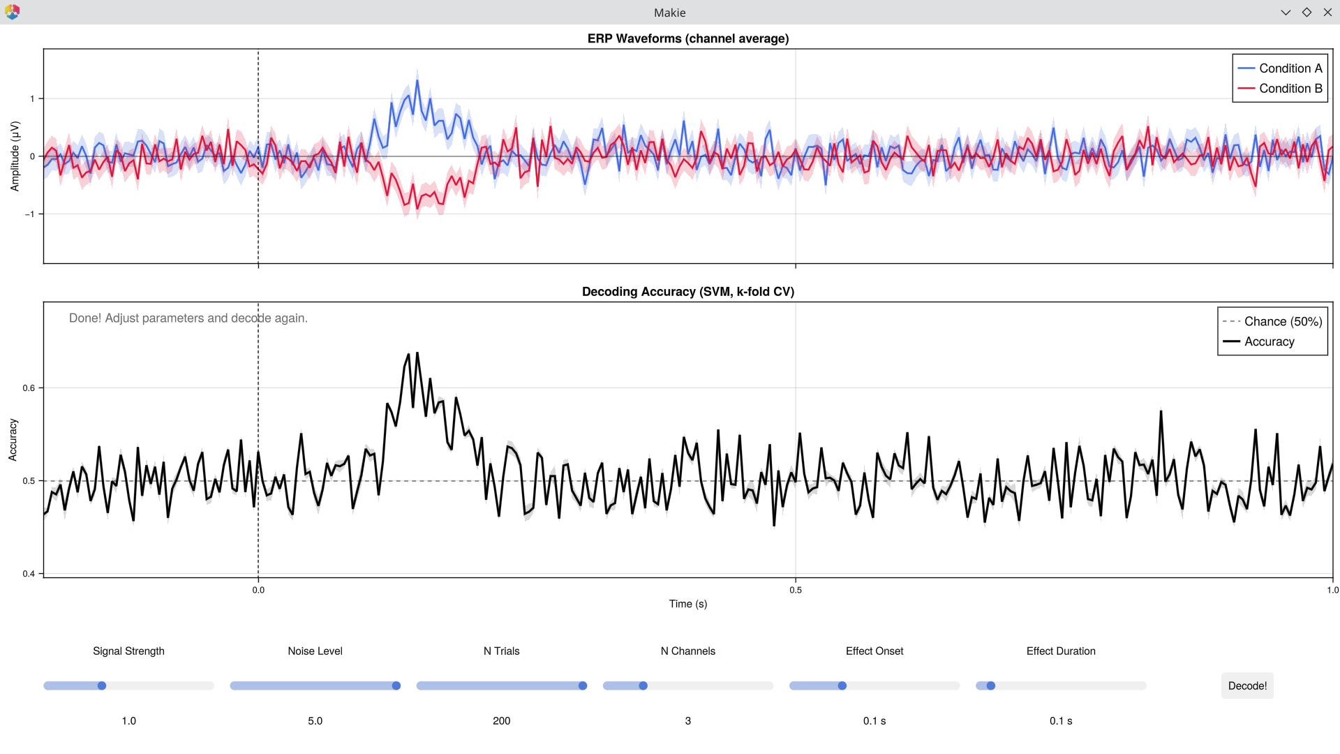
What it shows
| Element | Description |
|---|---|
| Blue/Red lines | Mean ERP waveforms for Condition A and B (channel average), with ±1 SE shading |
| Black line | Time-resolved SVM classification accuracy |
| Grey dashed line | 50% chance level — accuracy here means no decodable information |
The core insight: at each time point, a Support Vector Machine (SVM) classifier tries to distinguish the two conditions using the pattern of activity across channels. Accuracy above chance means the brain's response to the two conditions is reliably different at that moment.
Key Concepts
Multivariate vs. univariate: A t-test compares one channel at a time. MVPA considers the joint pattern across all channels simultaneously — exploiting spatial correlations that univariate methods miss. This is why more channels can improve decoding even when individual channels show weak effects.
Cross-validation: The data is split into training and test sets. The SVM learns the pattern from training data and is tested on data it has never seen. This prevents overfitting — being fooled by noise patterns that don't generalise.
Effect size and SNR: Signal Strength controls how different the two conditions are. With zero signal, accuracy bounces around 50% (chance). As signal increases, accuracy rises. But noise fights back — high noise can bury even a strong signal if you don't have enough trials.
Things to Try
Default settings: press Decode! — you should see accuracy rising above chance in the effect window.
Kill the signal: set Signal Strength = 0, decode → accuracy fluctuates around 50%. This is the null distribution.
Crank the signal: set Signal Strength = 3 → accuracy approaches 100%.
Multivariate advantage: set N Channels = 1, decode. Then set N Channels = 10, decode again — more channels = higher accuracy.
Trial count matters: set N Trials = 10 → noisy, unreliable curve. Set N Trials = 200 → smooth, stable curve.
Timing information: shift Effect Onset to 0.5 s → accuracy peak shifts to match. Change Duration to see the peak widen or narrow.
Controls
| Control | Range | Description |
|---|---|---|
| Signal Strength | 0–3 | Amplitude of the condition difference |
| Noise Level | 0.1–5 | Background noise amplitude |
| N Trials | 10–200 | Trials per condition |
| N Channels | 1–10 | Number of EEG channels (SVM features) |
| Effect Onset | −0.2–0.8 s | When the condition difference begins |
| Effect Duration | 0.05–0.8 s | How long the condition difference lasts |
| Decode! | button | Runs the SVM classification |
See Also
Simulate ERP — how trial averaging extracts signals from noise
Signal Example — Composition — signal composition and filtering
Signal Example — Time-Frequency — time-frequency analysis methods
Grootswagers, T., Wardle, S. G., & Carlson, T. A. (2017). Decoding dynamic brain patterns from evoked responses: a tutorial on multivariate pattern analysis applied to time series neuroimaging data. Journal of Cognitive Neuroscience, 29(4), 677–697.
Code
using EegFun
EegFun.signal_example_decoding()